gtregression supports a complete survival workflow:
describe the cohort, draw Kaplan-Meier curves, summarise observed
survival, compare groups, fit Cox or parametric survival models, check
assumptions, predict survival probabilities, visualise estimates, and
export publication-ready tables.
library(gtregression)
library(dplyr)

data("data_lungcancer", package = "gtregression")

lung_data <- data_lungcancer |>
  mutate(
    trt = factor(trt, levels = c(1, 2),
                 labels = c("Standard treatment", "Test treatment")),
    prior = factor(prior, levels = c(0, 10), labels = c("No", "Yes")),
    celltype = factor(
      celltype,
      levels = c("squamous", "smallcell", "adeno", "large"),
      labels = c("Squamous", "Small cell", "Adenocarcinoma", "Large cell")
    )
  )

attr(lung_data$time, "label") <- "Survival time"
attr(lung_data$status, "label") <- "Death status"
attr(lung_data$trt, "label") <- "Treatment group"
attr(lung_data$celltype, "label") <- "Cancer cell type"
attr(lung_data$karno, "label") <- "Karnofsky performance score"
attr(lung_data$age, "label") <- "Age"
attr(lung_data$prior, "label") <- "Prior therapy"

surv_exposures <- c("trt", "celltype", "karno", "age", "prior")
1. Describe The Cohort
Start with a baseline table. This helps readers understand the treatment groups before looking at survival curves or models.
lung_summary <- descriptive_table(
  data = lung_data,
  exposures = c("time", "status", "celltype", "karno", "age", "prior"),
  by = trt,
  statistic = c(time = "median", karno = "mean", age = "mean"),
  percent = column,
  show_overall = last
)

lung_summary$table
Characteristic |
Standard treatment, N=69 |
Test treatment, N=68 |
Overall, N=137 |
|---|---|---|---|
Survival time |
97.0 (25.0-153.0) |
52.5 (24.8-117.2) |
80.0 (25.0-144.0) |
Death status |
|||
0 |
5 (7.2%) |
4 (5.9%) |
9 (6.6%) |
1 |
64 (92.8%) |
64 (94.1%) |
128 (93.4%) |
Cancer cell type |
|||
Squamous |
15 (21.7%) |
20 (29.4%) |
35 (25.5%) |
Small cell |
30 (43.5%) |
18 (26.5%) |
48 (35.0%) |
Adenocarcinoma |
9 (13.0%) |
18 (26.5%) |
27 (19.7%) |
Large cell |
15 (21.7%) |
12 (17.6%) |
27 (19.7%) |
Karnofsky performance score |
59.2 (18.7) |
57.9 (21.4) |
58.6 (20.0) |
Age |
57.5 (10.8) |
59.1 (10.3) |
58.3 (10.5) |
Prior therapy |
|||
No |
48 (69.6%) |
49 (72.1%) |
97 (70.8%) |
Yes |
21 (30.4%) |
19 (27.9%) |
40 (29.2%) |
Categorical variables shown as n (%); percentages are by column. | |||
Continuous summaries: time = Median (IQR); karno = Mean (SD); age = Mean (SD). | |||
2. Show Observed Survival
Use km_plot() for the Kaplan-Meier curve. Add
risk_table = TRUE when the number at risk should appear
under the curve. When survival remains high, use ylim to
focus the y-axis, for example ylim = c(50, 100) with the
default percentage scale. Confidence intervals are shown as shaded bands
when conf.int = TRUE.
km_curve <- km_plot(
  data = lung_data,
  time = time,
  event = status,
  by = trt,
  break_time_by = 200,
  ylim = c(50, 100),
  title = "Kaplan-Meier Survival by Treatment"
)

km_curve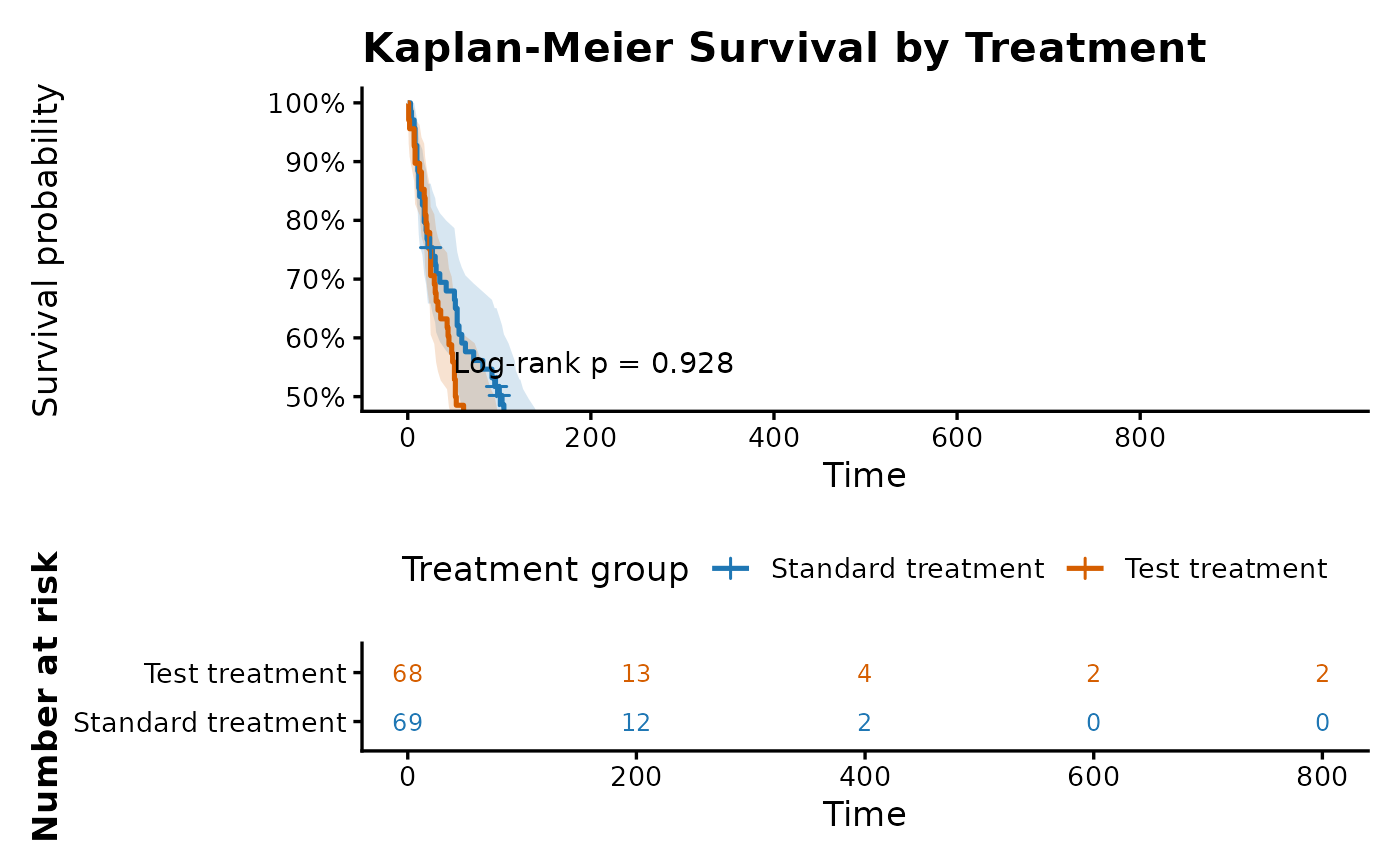
For multi-panel publication figures, make each Kaplan-Meier plot
lighter and let patchwork arrange the panels. A common
pattern is to remove the risk table, use short panel titles, reduce
title_size, and collect legends across panels.
km_trt_panel <- km_plot(
  data = lung_data,
  time = time,
  event = status,
  by = trt,
  risk_table = FALSE,
  break_time_by = 200,
  ylim = c(50, 100),
  title = "A. Treatment group",
  title_size = 10,
  title_face = plain,
  legend_position = bottom,
  base_size = 10
)

km_prior_panel <- km_plot(
  data = lung_data,
  time = time,
  event = status,
  by = prior,
  risk_table = FALSE,
  break_time_by = 200,
  ylim = c(50, 100),
  title = "B. Prior therapy",
  title_size = 10,
  title_face = plain,
  legend_position = bottom,
  base_size = 10
)

patchwork::wrap_plots(km_trt_panel, km_prior_panel, ncol = 2) +
  patchwork::plot_layout(guides = "collect") &
  ggplot2::theme(legend.position = "bottom")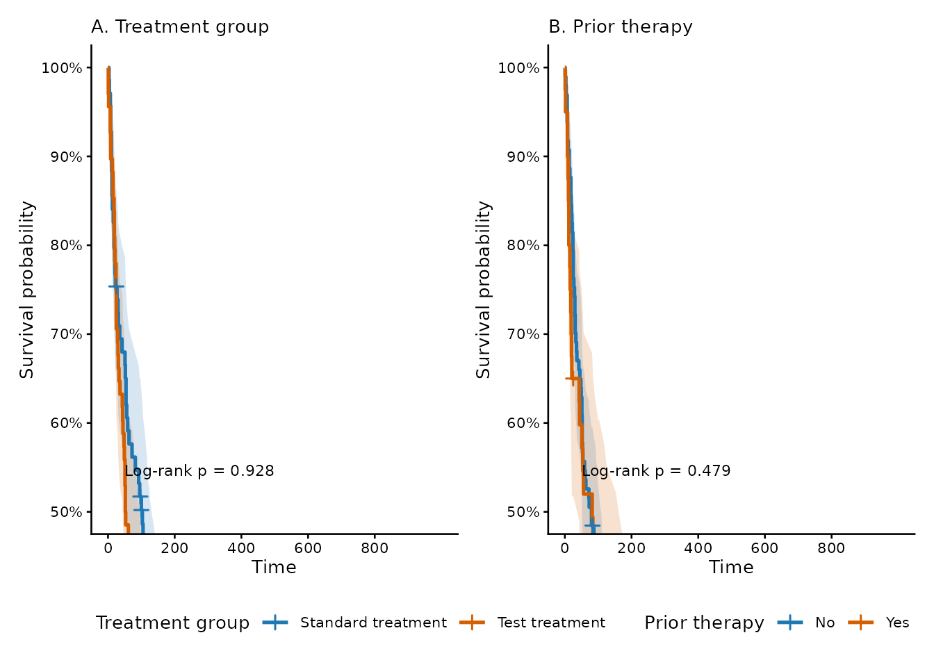
Use table summaries when readers need exact survival values.
survival_summary(
  data = lung_data,
  time = time,
  event = status,
  by = trt
)$tableGroup |
N |
Events |
Censored |
Median survival (95% CI) |
|---|---|---|---|---|
Standard treatment |
69 |
64 |
5 |
103.0 (59.0-132.0) |
Test treatment |
68 |
64 |
4 |
52.5 (44.0-95.0) |
Median survival is estimated using Kaplan-Meier methods. Not reached means survival did not fall to 50% during observed follow-up. | ||||
survival_prob(
  data = lung_data,
  time = time,
  event = status,
  by = trt,
  times = c(90, 180, 365)
)$tableGroup |
Time |
At risk |
Events |
Censored |
Survival probability (95% CI) |
|---|---|---|---|---|---|
Standard treatment |
90.0 |
37 |
31 |
1 |
54.7% (44.0%-67.9%) |
Standard treatment |
180.0 |
13 |
21 |
3 |
21.2% (13.2%-34.1%) |
Standard treatment |
365.0 |
4 |
8 |
1 |
7.1% (2.8%-18.0%) |
Test treatment |
90.0 |
25 |
42 |
2 |
38.0% (28.0%-51.6%) |
Test treatment |
180.0 |
14 |
9 |
1 |
23.3% (14.9%-36.3%) |
Test treatment |
365.0 |
6 |
7 |
1 |
11.0% (5.3%-22.7%) |
Survival probabilities are estimated using Kaplan-Meier methods. Events and censored counts are interval counts up to each requested time point. | |||||
rmst_table() reports restricted mean survival time up to
a chosen follow-up time. This is useful when an absolute survival-time
summary is easier to explain than a ratio measure.
rmst_table(
  data = lung_data,
  time = time,
  event = status,
  by = trt,
  tau = 365
)$tableGroup |
Tau |
N |
Events |
RMST (95% CI) |
RMST difference (95% CI) |
p-value |
|---|---|---|---|---|---|---|
Standard treatment |
365.0 |
69 |
64 |
119.0 (93.5-144.5) |
||
Test treatment |
365.0 |
68 |
64 |
112.4 (83.3-141.6) |
||
Difference (Test treatment - Standard treatment) |
365.0 |
-6.6 (-45.3-32.2) |
0.740 |
|||
RMST is restricted mean survival time up to tau. For two groups, the difference is the second group minus the first group. | ||||||
3. Compare Survival Curves
logrank_test() compares Kaplan-Meier curves. It is a
group comparison test, not an effect-size model.
logrank_test(
  data = lung_data,
  time = time,
  event = status,
  by = trt
)$tableGroup |
N |
Observed events |
Expected events |
|---|---|---|---|
Standard treatment |
69 |
64 |
64.50 |
Test treatment |
68 |
64 |
63.50 |
Log-rank test: chi-square = 0.01, df = 1, p-value = 0.928. This compares survival curves; use cox_reg() when a hazard ratio is needed. | |||
4. Fit Cox Regression
cox_reg() reports hazard ratios. Use
adjust_for to produce adjusted hazard ratios while keeping
the syntax aligned with multi_reg().
cox_crude <- cox_reg(
  data = lung_data,
  time = time,
  event = status,
  exposures = surv_exposures
)

cox_adjusted <- cox_reg(
  data = lung_data,
  time = time,
  event = status,
  exposures = c(trt, celltype, prior),
  adjust_for = c(age, karno)
)

cox_adjusted$table
Characteristic |
Adjusted HR (95% CI) |
p-value |
|---|---|---|
Treatment group |
||
Standard treatment |
Ref. |
|
Test treatment |
1.21 (0.84–1.74) |
0.307 |
Cancer cell type |
||
Squamous |
Ref. |
|
Small cell |
2.06 (1.26–3.39) |
0.004 |
Adenocarcinoma |
3.23 (1.82–5.74) |
<0.001 |
Large cell |
1.38 (0.80–2.37) |
0.244 |
Prior therapy |
||
No |
Ref. |
|
Yes |
0.96 (0.64–1.42) |
0.820 |
Abbreviations: HR = Hazard Ratio; CI = Confidence Interval. | ||
Ref. = reference category. | ||
Adjusted for Age and Karnofsky performance score | ||
Planned interactions use the same
interaction = exposure*modifier grammar as
multi_reg(). In the default exposure-by-exposure workflow,
supply the single exposure you want to interpret.
cox_interaction <- cox_reg(
  data = lung_data,
  time = time,
  event = status,
  exposures = trt,
  adjust_for = c(age, karno),
  interaction = trt*prior
)

cox_interaction$table
Characteristic |
Adjusted HR (95% CI) |
p-value |
|---|---|---|
Treatment group |
||
Standard treatment |
Ref. |
|
Test treatment |
1.52 (0.98–2.36) |
0.061 |
Treatment group: Test treatment x Prior therapy: Yes |
0.47 (0.21–1.06) |
0.070 |
Abbreviations: HR = Hazard Ratio; CI = Confidence Interval. | ||
Ref. = reference category. | ||
Adjusted for Age and Karnofsky performance score | ||
Model includes interaction term: trt*prior | ||
Check the proportional hazards assumption before treating Cox hazard ratios as final.
check_ph(cox_adjusted)$table## NULL5. Fit Parametric Survival Regression
surv_reg() fits accelerated failure time style
parametric survival models and reports time ratios. A time ratio above 1
suggests longer survival time; below 1 suggests shorter survival time,
conditional on the selected distribution.
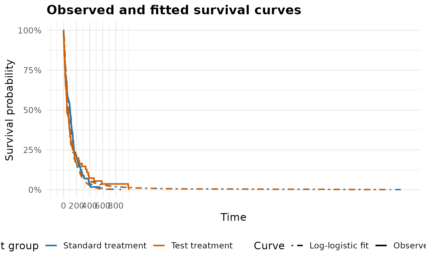
Before choosing the final distribution, compare candidate parametric models numerically and visually. Lower AIC/BIC is useful for screening; the fitted curve should also look reasonable against the Kaplan-Meier curve.
surv_model_compare(
  data = lung_data,
  time = time,
  event = status,
  exposures = c(trt, celltype, prior),
  adjust_for = c(age, karno),
  distributions = c(weibull, exponential, "log-normal", "log-logistic")
)$tableDistribution |
AIC |
BIC |
Log-likelihood |
Scale |
N |
Events |
Best AIC |
Best BIC |
|---|---|---|---|---|---|---|---|---|
loglogistic |
1,441.93 |
1,468.21 |
-711.96 |
0.58 |
137 |
128 |
Yes |
Yes |
lognormal |
1,447.29 |
1,473.57 |
-714.64 |
1.06 |
137 |
128 |
No |
No |
exponential |
1,448.32 |
1,471.68 |
-716.16 |
1.00 |
137 |
128 |
No |
No |
weibull |
1,449.11 |
1,475.39 |
-715.55 |
0.93 |
137 |
128 |
No |
No |
Lower AIC or BIC indicates better relative fit among the compared distributions. Use model fit statistics with clinical judgment and visual checks. | ||||||||
plot_surv_fit(
  data = lung_data,
  time = time,
  event = status,
  by = trt,
  adjust_for = c(age, karno),
  distributions = c(weibull, "log-logistic"),
  break_time_by = 200
)
After selecting a distribution, fit crude and adjusted publication-ready tables.
surv_crude <- surv_reg(
  data = lung_data,
  time = time,
  event = status,
  exposures = surv_exposures,
  distribution = loglogistic
)

surv_adjusted <- surv_reg(
  data = lung_data,
  time = time,
  event = status,
  exposures = c(trt, celltype, prior),
  adjust_for = c(age, karno),
  distribution = loglogistic,
  model_stats = TRUE
)

surv_adjusted$table
Characteristic |
Adjusted Time Ratio (95% CI) |
p-value |
|---|---|---|
Treatment group |
||
Standard treatment |
Ref. |
|
Test treatment |
0.95 (0.66–1.37) |
0.771 |
Cancer cell type |
||
Squamous |
Ref. |
|
Small cell |
0.51 (0.31–0.81) |
0.005 |
Adenocarcinoma |
0.48 (0.28–0.80) |
0.005 |
Large cell |
1.01 (0.60–1.71) |
0.968 |
Prior therapy |
||
No |
Ref. |
|
Yes |
1.07 (0.71–1.62) |
0.740 |
Abbreviations: Time Ratio = exponentiated accelerated failure time coefficient; CI = Confidence Interval. | ||
Distribution: loglogistic. | ||
Ref. = reference category. | ||
Adjusted for Age and Karnofsky performance score | ||
surv_adjusted$model_stats## model distribution AIC BIC logLik scale events n
## 1 trt loglogistic 1449.511 1464.111 -719.7554 0.6186080 128 137
## 2 celltype loglogistic 1438.331 1458.771 -712.1656 0.5796411 128 137
## 3 prior loglogistic 1449.486 1464.086 -719.7429 0.6178590 128 137Parametric survival models use the same interaction grammar and display Adjusted Time Ratio (95% CI) when adjustment or multivariable modelling is used.
surv_interaction <- surv_reg(
  data = lung_data,
  time = time,
  event = status,
  exposures = trt,
  adjust_for = c(age, karno),
  interaction = trt*prior,
  distribution = loglogistic
)

surv_interaction$table
Characteristic |
Adjusted Time Ratio (95% CI) |
p-value |
|---|---|---|
Treatment group |
||
Standard treatment |
Ref. |
|
Test treatment |
0.84 (0.55–1.30) |
0.444 |
Treatment group: Test treatment x Prior therapy: Yes |
1.52 (0.66–3.47) |
0.323 |
Abbreviations: Time Ratio = exponentiated accelerated failure time coefficient; CI = Confidence Interval. | ||
Distribution: loglogistic. | ||
Ref. = reference category. | ||
Adjusted for Age and Karnofsky performance score | ||
Model includes interaction term: trt*prior | ||
6. Predict Survival Probabilities
surv_predict() turns a fitted parametric survival model
into predicted survival probabilities at selected follow-up times for a
profile.
surv_predict(
  model = surv_adjusted$models$trt,
  newdata = data.frame(
    trt = factor("Test treatment", levels = levels(lung_data$trt)),
    age = 60,
    karno = 70
  ),
  times = c(90, 180, 365)
)$tableProfile |
trt |
age |
karno |
Time |
Predicted survival |
Model distribution |
|---|---|---|---|---|---|---|
1 |
Test treatment |
60 |
70 |
90.0 |
54.5% |
loglogistic |
1 |
Test treatment |
60 |
70 |
180.0 |
28.1% |
loglogistic |
1 |
Test treatment |
60 |
70 |
365.0 |
11.1% |
loglogistic |
Model-based predictions from a parametric survival regression model. Distribution: loglogistic. Predictions depend on the supplied profile and model specification. | ||||||
7. Visualise And Export Model Results
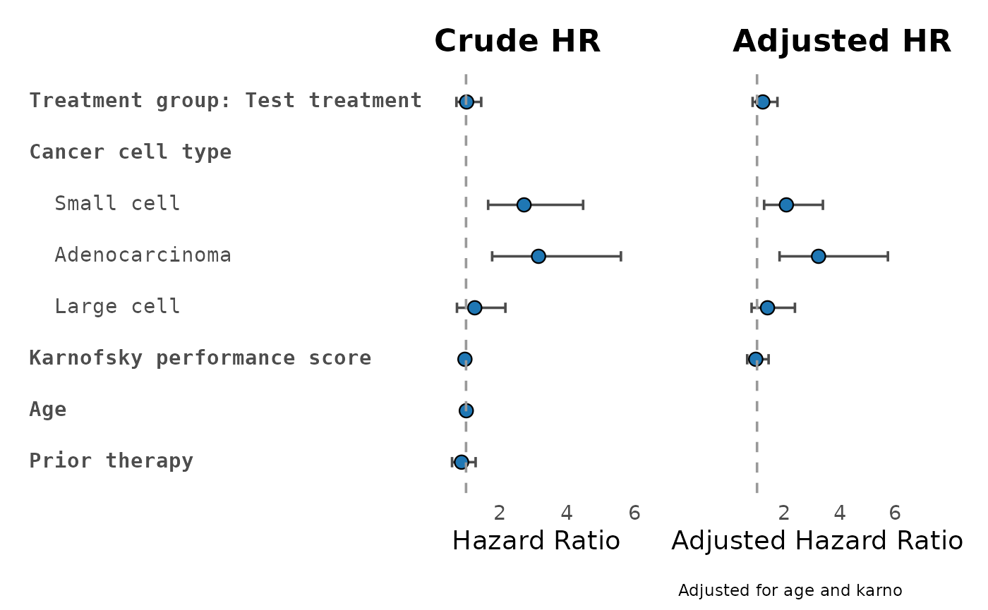
The survival model outputs work with the same downstream tools used for other regression tables.
plot_reg_combine(
  cox_crude,
  cox_adjusted,
  show_ref = FALSE,
  title_uni = "Crude HR",
  title_multi = "Adjusted HR"
)
surv_forest_data <- forest_df(cox_crude, cox_adjusted, desc = lung_summary)

forest_reg(
  surv_forest_data,
  xlim = list(c(0.25, 8), c(0.25, 8)),
  ticks_at = list(c(0.5, 1, 2, 4, 8), c(0.5, 1, 2, 4, 8)),
  quiet = TRUE
)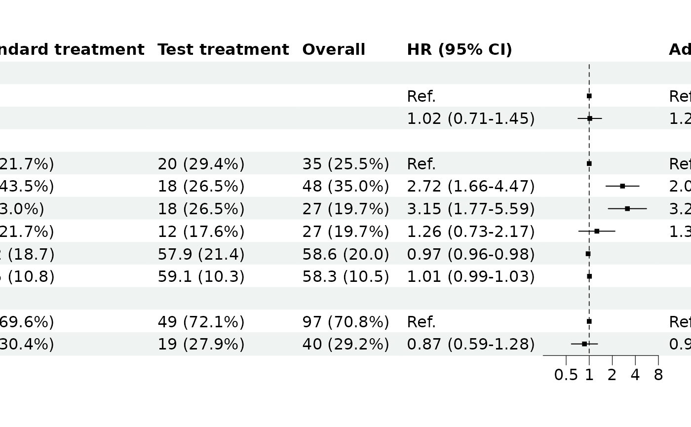
If forest plot x-axis labels overlap, set xlim and
ticks_at. If the confidence-interval plot panel is too
narrow or too wide, tune ci_col_width. For very wide
descriptive-plus-crude-plus-adjusted tables, export using a wider
graphics device or Word canvas.
Survival Workflow Map
| Task | Function |
|---|---|
| Kaplan-Meier curve | km_plot() |
| Number at risk | km_risk_table() |
| Median survival | survival_summary() |
| Survival quantiles | survival_quantiles() |
| Fixed-time survival probability | survival_prob() |
| Restricted mean survival time | rmst_table() |
| Compare KM curves | logrank_test() |
| Cox hazard ratios | cox_reg() |
| Cox PH check | check_ph() |
| Parametric time ratios | surv_reg() |
| Compare parametric distributions | surv_model_compare() |
| Plot fitted parametric curves | plot_surv_fit() |
| Predict survival probabilities | surv_predict() |
| Model plots and forest tables |
plot_reg(), plot_reg_combine(),
forest_df(), forest_reg()
|