Diagnostics and Model Selection

Before the final table goes into a manuscript, check the model. These helpers keep diagnostics close to the regression workflow. They are screening aids: interpret them with the study design, clinical or subject-matter judgement, and the diagnostics from the fitted model.

library(gtregression)
library(dplyr)

data("data_birthwt", package = "gtregression")

birthwt_data <- data_birthwt |>
  mutate(
    race = factor(race, levels = c(1, 2, 3),
                  labels = c("White", "Black", "Other")),
    smoke = factor(smoke, levels = c(0, 1), labels = c("No", "Yes")),
    ht = factor(ht, levels = c(0, 1), labels = c("No", "Yes")),
    ui = factor(ui, levels = c(0, 1), labels = c("No", "Yes")),
    low = factor(low, levels = c(0, 1), labels = c("Normal BW", "Low BW")),
    ptl_cat = factor(ifelse(ptl > 0, "Yes", "No"), levels = c("No", "Yes"))
  )

exposures <- c("age", "lwt", "race", "smoke", "ht", "ui", "ptl_cat")

Convergence Screening

Use check_convergence() before interpreting model estimates, especially for log-binomial and small or sparse binary-outcome models. A non-converged model is a fitting warning, not a finding.

check_convergence(
  data = birthwt_data,
  exposures = exposures,
  outcome = low,
  approach = logit,
  multivariate = TRUE,
  format = gt
)

Convergence check
Exposure	Model	Converged	Max fitted value
age + lwt + race + smoke + ht + ui + ptl_cat	logit	Yes	0.880
Screening aid only; inspect non-convergence, impossible fitted values, and model specification before interpreting estimates.

For risk-ratio workflows, this same check helps users decide whether a log-binomial model fitted cleanly or whether a robust Poisson approach may be a more practical sensitivity analysis.

check_convergence(
  data = birthwt_data,
  exposures = c("smoke", "ht", "ui", "ptl_cat"),
  outcome = low,
  approach = logbinomial,
  multivariate = TRUE,
  format = flextable
)

Convergence check

Exposure	Model	Converged	Max fitted value
smoke + ht + ui + ptl_cat	logbinomial	No
Screening aid only; inspect non-convergence, impossible fitted values, and model specification before interpreting estimates.

Collinearity Screening

check_collinearity() reports VIF-style diagnostics for multivariable models. High VIF values are prompts to inspect coding, overlap between predictors, and the scientific purpose of the model.

birthwt_multi <- multi_reg(
  data = birthwt_data,
  outcome = low,
  exposures = exposures,
  approach = logit
)

check_collinearity(birthwt_multi, format = gt)

Collinearity check
Variable	VIF	Interpretation
age	1.04	No collinearity
lwt	1.14	No collinearity
race	1.11	No collinearity
smoke	1.16	No collinearity
ht	1.08	No collinearity
ui	1.02	No collinearity
ptl_cat	1.05	No collinearity
Screening aid only; interpret VIF with model purpose, coding choices, sample size, and subject-matter knowledge.

Adjusted-mode multi_reg() objects contain one model per exposure. The collinearity output keeps that list structure so each model can be inspected separately.

birthwt_adjusted <- multi_reg(
  data = birthwt_data,
  outcome = low,
  exposures = c("smoke", "ht", "ui", "ptl_cat"),
  adjust_for = c("age", "lwt", "race"),
  approach = logit
)

check_collinearity(birthwt_adjusted, format = tibble)

## $smoke
## # A tibble: 4 × 3
##   Variable   VIF Interpretation 
##   <chr>    <dbl> <chr>          
## 1 smoke     1.14 No collinearity
## 2 age       1.03 No collinearity
## 3 lwt       1.06 No collinearity
## 4 race      1.1  No collinearity
## 
## $ht
## # A tibble: 4 × 3
##   Variable   VIF Interpretation 
##   <chr>    <dbl> <chr>          
## 1 ht        1.07 No collinearity
## 2 age       1.02 No collinearity
## 3 lwt       1.14 No collinearity
## 4 race      1.03 No collinearity
## 
## $ui
## # A tibble: 4 × 3
##   Variable   VIF Interpretation 
##   <chr>    <dbl> <chr>          
## 1 ui        1.01 No collinearity
## 2 age       1.03 No collinearity
## 3 lwt       1.07 No collinearity
## 4 race      1.04 No collinearity
## 
## $ptl_cat
## # A tibble: 4 × 3
##   Variable   VIF Interpretation 
##   <chr>    <dbl> <chr>          
## 1 ptl_cat   1.03 No collinearity
## 2 age       1.05 No collinearity
## 3 lwt       1.07 No collinearity
## 4 race      1.04 No collinearity

Model Fit Plots

plot_model_fit() turns fitted models into quick diagnostic plots. It accepts raw lm() and glm() objects, and it also works with models saved inside uni_reg() and multi_reg() results.

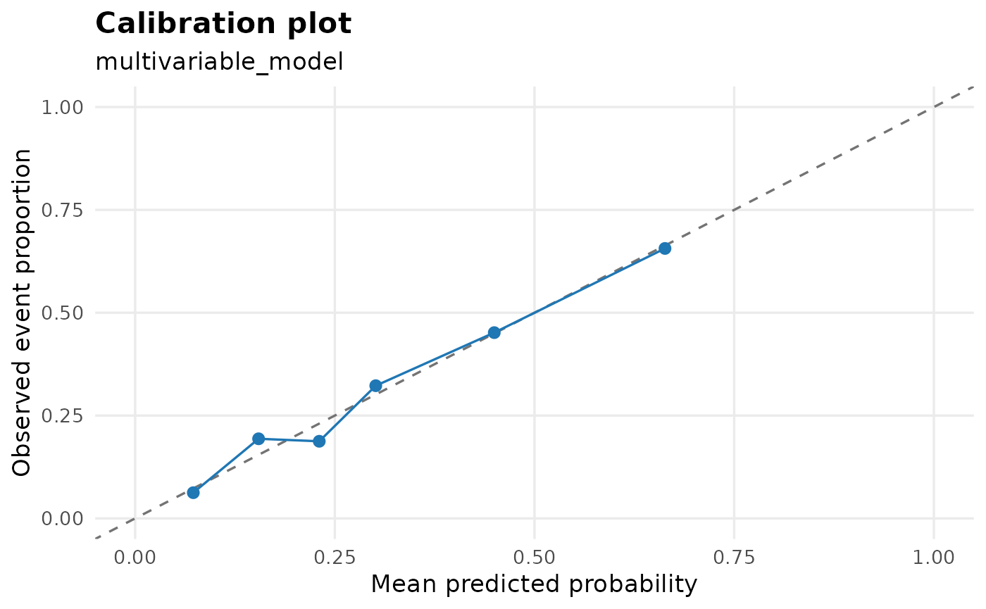
For logistic regression, the calibration plot compares predicted probabilities with observed event proportions. Points close to the diagonal line suggest that the model predictions are reasonably aligned with the observed data. Calibration is usually most useful for multivariable models because predicted probabilities vary across many people.

plot_model_fit(
  birthwt_multi,
  type = calibration,
  bins = 6
)

When a uni_reg() object contains several models, use model_name to choose the exposure you want to inspect. For a simple binary exposure, calibration may only show two points because the model has only two fitted probabilities; in that situation, residual and influence plots are usually more useful.

birthwt_uni <- uni_reg(
  data = birthwt_data,
  outcome = low,
  exposures = c("age", "lwt", "smoke"),
  approach = logit
)

plot_model_fit(
  birthwt_uni,
  model_name = smoke,
  type = residual
)

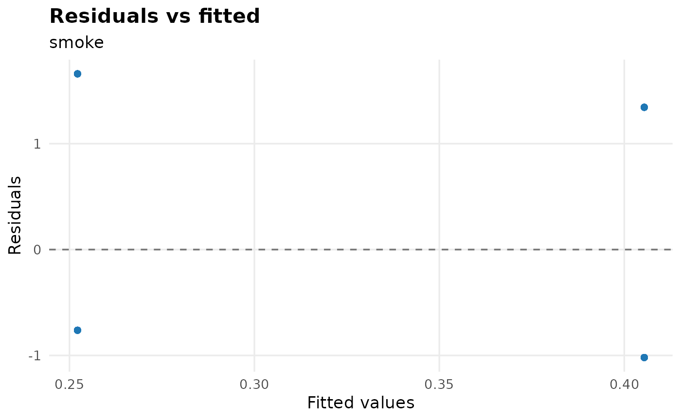
For logistic models, residual plots often form two visible bands. That is a normal consequence of a 0/1 outcome and should be interpreted as a screening plot rather than a linear-model residual plot.

For linear regression, type = all shows the classic residual, Q-Q, scale-location, and Cook’s distance views.

fit_lm <- lm(bwt ~ age + lwt, data = birthwt_data)
plot_model_fit(fit_lm)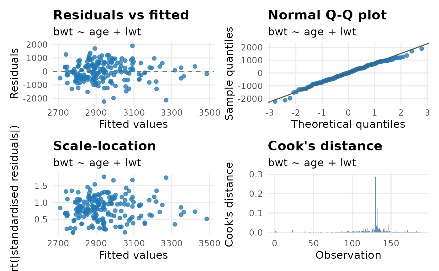

Proportional Hazards Screening

For Cox models, use check_ph() before treating hazard ratios as final. It reports Schoenfeld residual tests from survival::cox.zph(), including a global test. Small p-values suggest possible non-proportional hazards and should be reviewed with plots, follow-up pattern, and clinical judgement.

data("data_lungcancer", package = "gtregression")

lung_data <- data_lungcancer |>
  mutate(
    trt = factor(trt, levels = c(1, 2),
                 labels = c("Standard treatment", "Test treatment")),
    prior = factor(prior, levels = c(0, 10), labels = c("No", "Yes")),
    celltype = factor(
      celltype,
      levels = c("squamous", "smallcell", "adeno", "large"),
      labels = c("Squamous", "Small cell", "Adenocarcinoma", "Large cell")
    )
  )

cox_fit <- cox_reg(
  data = lung_data,
  time = time,
  event = status,
  exposures = c(trt, celltype, prior),
  adjust_for = c(age, karno)
)

check_ph(cox_fit, format = gt)

Proportional hazards check
Model	Term	Test	Chi-square	df	p-value	Interpretation
trt	trt	Term	0.28	1	0.594	No evidence of PH violation
trt	age	Term	2.10	1	0.147	No evidence of PH violation
trt	karno	Term	12.00	1	<0.001	Possible PH violation
trt	GLOBAL	Global	19.10	3	<0.001	Possible PH violation
celltype	celltype	Term	14.15	3	0.003	Possible PH violation
celltype	age	Term	1.99	1	0.158	No evidence of PH violation
celltype	karno	Term	14.77	1	<0.001	Possible PH violation
celltype	GLOBAL	Global	30.18	5	<0.001	Possible PH violation
prior	prior	Term	1.87	1	0.171	No evidence of PH violation
prior	age	Term	2.18	1	0.140	No evidence of PH violation
prior	karno	Term	13.31	1	<0.001	Possible PH violation
prior	GLOBAL	Global	22.29	3	<0.001	Possible PH violation
Screening aid only. Small p-values suggest possible non-proportional hazards; interpret with Schoenfeld residual plots, follow-up pattern, clinical context, and model purpose. alpha = 0.05; transform = km.

Use format = tibble when you want to inspect or filter the diagnostic results.

check_ph(cox_fit, transform = rank, format = tibble)

## # A tibble: 12 × 7
##    Model    Term     Test   Chi.square    df   p.value Interpretation           
##    <chr>    <chr>    <chr>       <dbl> <dbl>     <dbl> <chr>                    
##  1 trt      trt      Term        0.278     1 0.598     No evidence of PH violat…
##  2 trt      age      Term        2.04      1 0.153     No evidence of PH violat…
##  3 trt      karno    Term       12.6       1 0.000377  Possible PH violation    
##  4 trt      GLOBAL   Global     19.7       3 0.000191  Possible PH violation    
##  5 celltype celltype Term       14.3       3 0.00249   Possible PH violation    
##  6 celltype age      Term        1.93      1 0.164     No evidence of PH violat…
##  7 celltype karno    Term       15.4       1 0.0000877 Possible PH violation    
##  8 celltype GLOBAL   Global     30.6       5 0.0000114 Possible PH violation    
##  9 prior    prior    Term        1.92      1 0.166     No evidence of PH violat…
## 10 prior    age      Term        2.13      1 0.145     No evidence of PH violat…
## 11 prior    karno    Term       14.0       1 0.000187  Possible PH violation    
## 12 prior    GLOBAL   Global     23.0       3 0.0000401 Possible PH violation

Stepwise Model Selection

compare_models() is for prespecified candidate models that have already been fitted with gtregression. It answers a different question from stepwise selection: “How do these planned models compare?” The inputs should be multi_reg(), cox_reg(), or surv_reg() outputs, not raw lm(), glm(), coxph(), or survreg() objects. This keeps the workflow consistent with the publication-ready tables created by the package.

logit_m0 <- multi_reg(
  data = birthwt_data,
  outcome = low,
  exposures = smoke,
  approach = logit
)

logit_m1 <- multi_reg(
  data = birthwt_data,
  outcome = low,
  exposures = c(smoke, age, lwt),
  approach = logit
)

logit_m2 <- multi_reg(
  data = birthwt_data,
  outcome = low,
  exposures = c(smoke, age, lwt, race, ht, ui),
  approach = logit
)

logit_model_comparison <- compare_models(
  logit_m0,
  logit_m1,
  logit_m2,
  model_names = c(
    "Smoking only",
    "Add age and weight",
    "Full clinical model"
  ),
  primary_exposure = smoke,
  format = gt
)

logit_model_comparison$table

Model comparison
Model	Variables	N	Parameters	AIC	BIC	Best AIC	Best BIC	Log-likelihood	LR chi-square	df	p-value	Primary estimate	Change from first
Smoking only	smoke	189	2	233.80	240.29	No	Yes	-114.90				2.02	0.00%
Add age and weight	smoke + age + lwt	189	4	230.88	243.85	No	No	-111.44	6.93	2	0.031	1.96	-4.73%
Full clinical model	smoke + age + lwt + race + ht + ui	189	8	219.95	245.88	Yes	No	-101.97	18.93	4	<0.001	2.79	45.95%
Comparison status: Same analysis sample. Same analysis sample; assessed using retained model row identifiers. Nested-model status: sequential models are nested.
Compare prespecified candidate models; lower AIC or BIC indicates better relative fit among the compared models. Models were fitted to the same analysis sample. AIC, BIC, log-likelihood and likelihood-ratio tests may be interpreted as formal model-comparison statistics when the models are nested as required. Primary estimate change is calculated on the coefficient/log-effect scale before exponentiation and can help assess robustness across candidate models.

The table reports N, number of parameters, AIC, BIC, log-likelihood, and likelihood-ratio comparisons when nested = TRUE. Lower AIC or BIC identifies better relative fit among the compared models. When primary_exposure is supplied, the table also tracks that effect estimate and the percentage change across models.

compare_models() automatically checks whether the candidate models appear to use the same analysis sample. It uses retained row identifiers when the fitted model stores them; otherwise it compares N and event counts. If the models use different complete-case samples, the table still displays AIC, BIC, log-likelihood, and likelihood-ratio statistics for transparency, but the footer warns that these values should not be interpreted as formal model-selection criteria across different datasets. In that situation, use the primary exposure estimate, percentage change, confidence intervals, and clinical or epidemiological reasoning to judge robustness.

For Cox and parametric survival models, fit the candidate models with cox_reg() or surv_reg() first. compare_models() then keeps survival-specific columns such as events and Cox concordance.

cox_m0 <- cox_reg(
  data = lung_data,
  time = time,
  event = status,
  exposures = trt
)

cox_m1 <- cox_reg(
  data = lung_data,
  time = time,
  event = status,
  exposures = trt,
  adjust_for = c(age, karno)
)

cox_m2 <- cox_reg(
  data = lung_data,
  time = time,
  event = status,
  exposures = c(trt, age, karno, celltype, prior),
  multivariable = TRUE
)

cox_model_comparison <- compare_models(
  list(
    "Treatment only" = cox_m0,
    "Add age and performance" = cox_m1,
    "Full clinical model" = cox_m2
  ),
  primary_exposure = trt,
  format = gt
)

cox_model_comparison$table

Model comparison
Model	Variables	N	Events	Parameters	AIC	BIC	Best AIC	Best BIC	Log-likelihood	LR chi-square	df	p-value	Concordance	Primary estimate	Change from first
Treatment only	trt	137	128	1	1012.89	1015.74	No	No	-505.44				0.525	1.02	0.00%
Add age and performance	trt + age + karno	137	128	3	973.76	982.31	No	Yes	-483.88	43.13	2	<0.001	0.712	1.21	968.31%
Full clinical model	trt + age + karno + celltype + prior	137	128	7	962.79	982.76	Yes	No	-474.40	18.96	4	<0.001	0.736	1.34	1561.45%
Comparison status: Same analysis sample. Same analysis sample; assessed using retained model row identifiers. Nested-model status: sequential models are nested.
Compare prespecified candidate models; lower AIC or BIC indicates better relative fit among the compared models. Models were fitted to the same analysis sample. AIC, BIC, log-likelihood and likelihood-ratio tests may be interpreted as formal model-comparison statistics when the models are nested as required. Primary estimate change is calculated on the coefficient/log-effect scale before exponentiation and can help assess robustness across candidate models.

select_models() compares candidate models step by step. It is useful for exploration, teaching, and sensitivity checks. It should not replace a planned model based on study design or a causal framework.

selected <- select_models(
  data = birthwt_data,
  outcome = low,
  exposures = exposures,
  approach = logit,
  direction = forward,
  format = gt
)

selected$table

Stepwise model selection
Model	Selected variables	Predictors	AIC	BIC	Log-likelihood	deviance	Best AIC
1	Intercept only	0	236.67	239.91	-117.34	234.67	No
2	ptl_cat	1	225.90	232.38	-110.95	221.90	No
3	ptl_cat + age	2	223.30	233.02	-108.65	217.30	No
4	ptl_cat + age + ht	3	221.12	234.09	-106.56	213.12	No
5	ptl_cat + age + ht + lwt	4	217.43	233.64	-103.72	207.43	No
6	ptl_cat + age + ht + lwt + ui	5	217.15	236.60	-102.58	205.15	Yes
Selection direction: forward.
Screening aid only; compare candidate models with study design, clinical or subject-matter judgement, and model diagnostics.

The selected direction is recorded in the formatted table footer. Backward and both-direction searches are available using the same interface.

select_models(
  data = birthwt_data,
  outcome = low,
  exposures = exposures,
  approach = logit,
  direction = backward,
  format = tibble
)$results_table

## # A tibble: 2 × 9
##   model_id formula          model_terms n_predictors   AIC   BIC logLik deviance
##      <int> <chr>            <chr>              <int> <dbl> <dbl>  <dbl>    <dbl>
## 1        1 low ~ age + lwt… age + lwt …            7  215.  244.  -98.4     197.
## 2        2 low ~ lwt + rac… lwt + race…            6  214.  240.  -98.9     198.
## # ℹ 1 more variable: selected_vars <chr>

select_models(
  data = birthwt_data,
  outcome = low,
  exposures = exposures,
  approach = logit,
  direction = both,
  format = tibble
)$results_table

## # A tibble: 6 × 9
##   model_id formula          model_terms n_predictors   AIC   BIC logLik deviance
##      <int> <chr>            <chr>              <int> <dbl> <dbl>  <dbl>    <dbl>
## 1        1 low ~ 1          Intercept …            0  237.  240.  -117.     235.
## 2        2 low ~ ptl_cat    ptl_cat                1  226.  232.  -111.     222.
## 3        3 low ~ ptl_cat +… ptl_cat + …            2  223.  233.  -109.     217.
## 4        4 low ~ ptl_cat +… ptl_cat + …            3  221.  234.  -107.     213.
## 5        5 low ~ ptl_cat +… ptl_cat + …            4  217.  234.  -104.     207.
## 6        6 low ~ ptl_cat +… ptl_cat + …            5  217.  237.  -103.     205.
## # ℹ 1 more variable: selected_vars <chr>

What To Inspect

• check_convergence(): convergence status and maximum fitted probabilities. Use format = gt or format = flextable for viewing tables.
• check_collinearity(): VIF and interpretation. Nested model outputs keep their list structure when formatted.
• plot_model_fit(): residual, calibration, observed-versus-predicted, and influence plots for lm/glm models and stored uni_reg() / multi_reg() fitted models.
• check_ph(): Schoenfeld residual proportional hazards tests for Cox models, including term-level and global tests.
• compare_models(): AIC, BIC, log-likelihood, likelihood-ratio tests, sample size, events for survival models, and optional primary-exposure tracking for gtregression candidate models.
• select_models(): $results_table, $best_model, $all_models, and $direction; $table is added when format = gt or format = flextable.