Plot model-fit diagnostics — plot_model

Visualise model fit for fitted regression models and models stored inside uni_reg() or multi_reg() results.

Usage

plot_model_fit(
  model,
  model_name = NULL,
  type = c("auto", "all", "residual", "qq", "scale_location", "cooks",
    "observed_predicted", "calibration"),
  bins = 10,
  base_size = 13
)

Arguments

model: A fitted lm or glm model, or a uni_reg() / multi_reg() result.
model_name: Optional model name to select when model contains multiple fitted models. Quoted and bare names are accepted.
type: Plot type. One of "auto", "all", "residual", "qq", "scale_location", "cooks", "observed_predicted", or "calibration". Quoted and bare values are accepted.
bins: Number of groups used for binomial calibration plots.
base_size: Base font size for the plot theme.

Value

A ggplot2 object for a single plot, or a patchwork object when multiple diagnostics are requested.

Details

plot_model_fit() is a visual check of how a fitted model behaves, not a formal model-selection rule. For survival models, use check_ph() for Cox proportional hazards diagnostics and plot_surv_fit() for parametric survival model fit.

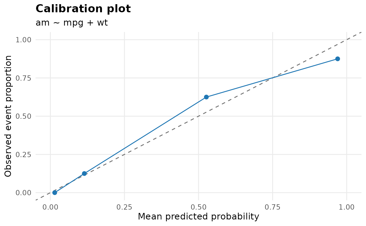
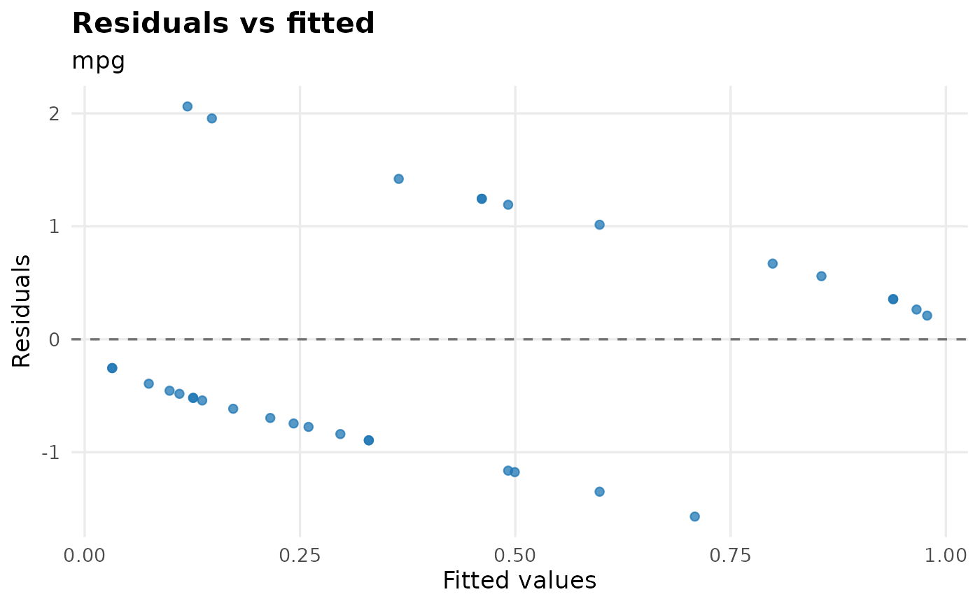
For binomial models, type = "calibration" compares grouped predicted probabilities with observed event proportions. This is most informative for multivariable models, where predictions vary across many patients. A univariable binary predictor may produce only two calibration points; that is expected and simply reflects the two fitted probabilities in the model. Logistic residual plots often show two bands because the outcome is coded as event/non-event.

Examples

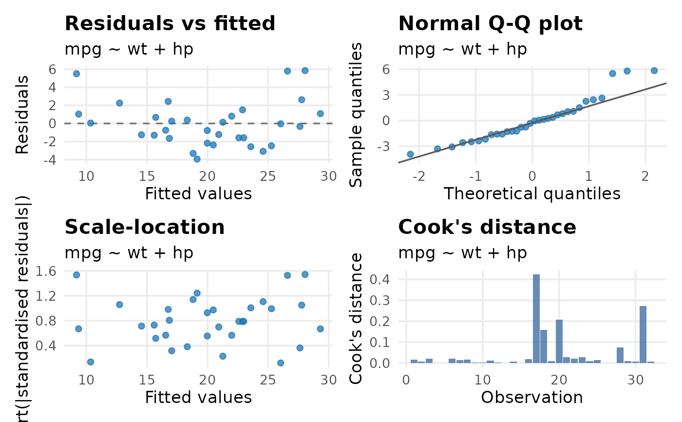
fit_lm <- lm(mpg ~ wt + hp, data = mtcars)
plot_model_fit(fit_lm)


fit_glm <- glm(am ~ mpg + wt, data = mtcars, family = binomial())
plot_model_fit(fit_glm, type = calibration, bins = 4)


uni_fit <- uni_reg(mtcars, am, c(mpg, wt), approach = logit)
plot_model_fit(uni_fit, model_name = mpg, type = residual)