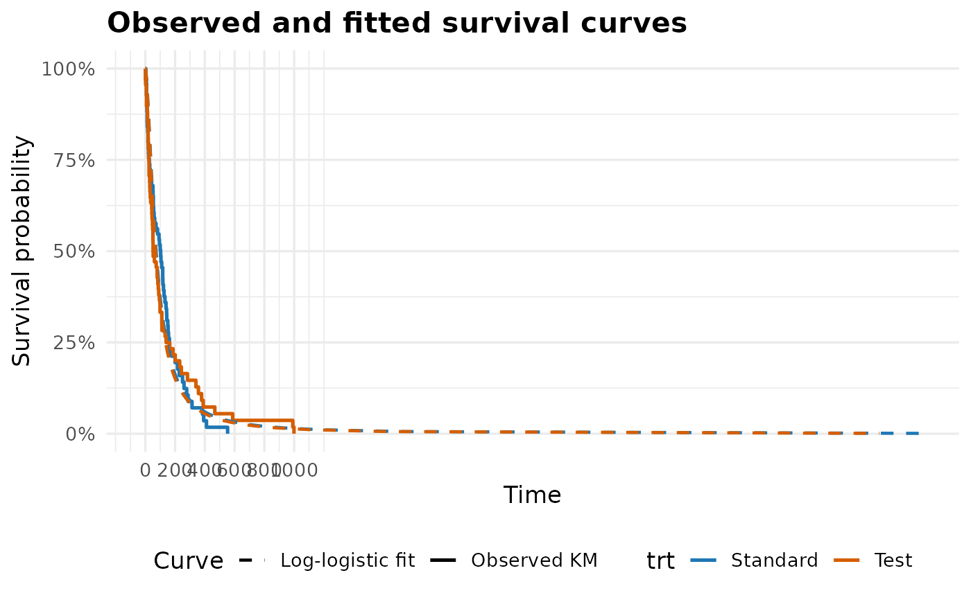
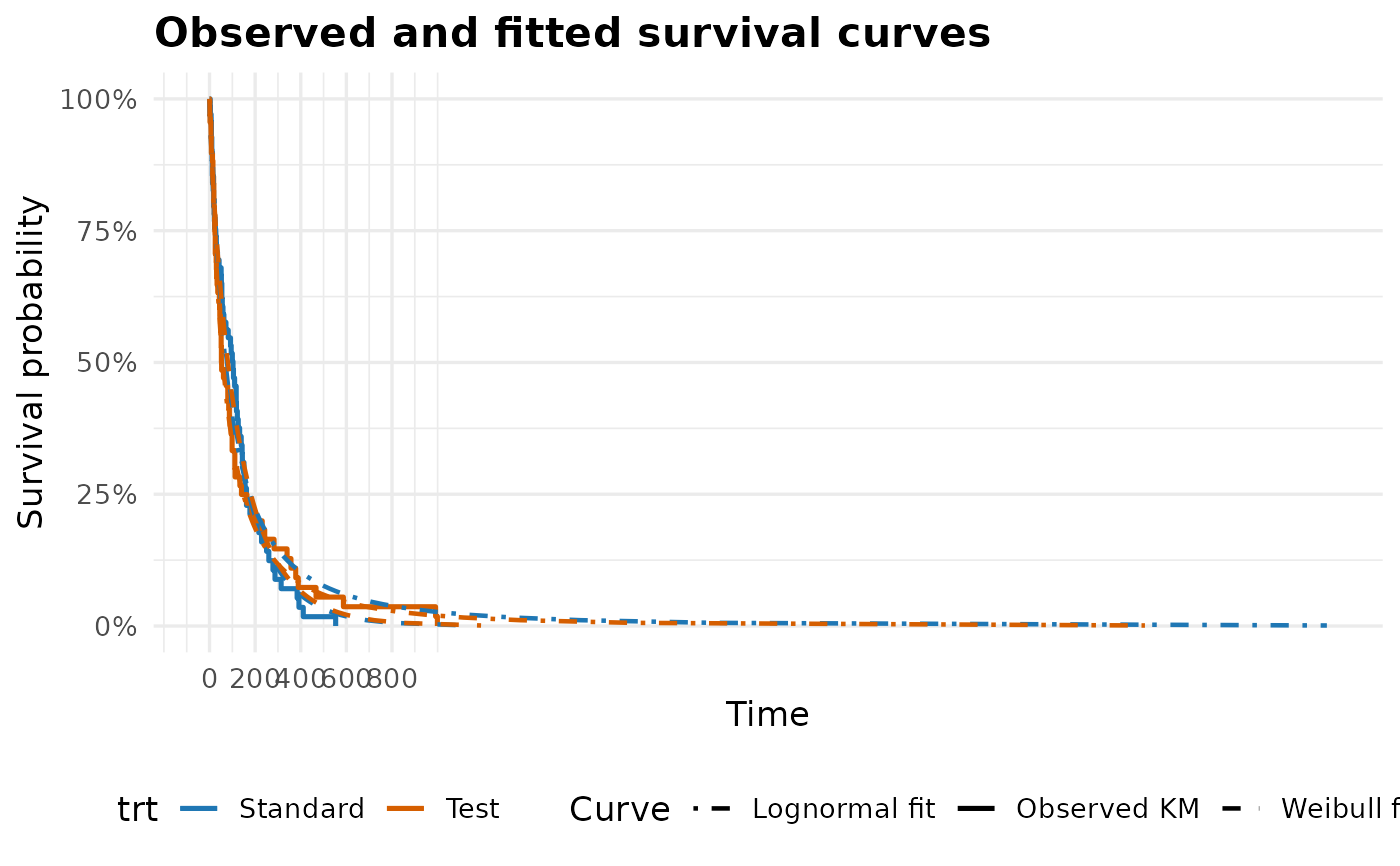
Plot observed and fitted parametric survival curves — plot_surv

Compare the observed Kaplan-Meier survival curve with fitted parametric survival curves from survival::survreg().

Usage

plot_surv_fit(
  data,
  time,
  event,
  by = NULL,
  adjust_for = NULL,
  distributions = c("weibull", "exponential", "lognormal", "loglogistic"),
  break_time_by = NULL,
  xlim = NULL,
  xlab = "Time",
  ylab = "Survival probability",
  title = NULL,
  legend_title = NULL,
  palette = NULL,
  base_size = 13,
  n_points = 200
)

Arguments

data: A data.frame containing survival time, event status, and optional grouping or adjustment variables.
time: Survival follow-up time. Quoted and bare names are accepted.
event: Event indicator. Quoted and bare names are accepted. Numeric 0/1, numeric 1/2, logical, character, and factor variables are accepted. For two-level character or factor variables, the second level is treated as the event.
by: Optional grouping variable for observed and fitted curves. Quoted and bare names are accepted.
adjust_for: Optional character vector of adjustment variables included in the fitted parametric model. Fitted curves are predicted at typical adjustment values.
distributions: Parametric survival distributions to overlay. One or more of "weibull", "exponential", "lognormal", or "loglogistic". Quoted and bare values are accepted. Common spellings such as "log-normal" and "log-logistic" are also accepted.
break_time_by: Optional numeric interval for x-axis breaks. If NULL, breaks are chosen automatically.
xlim: Optional numeric vector of length 2 specifying x-axis limits.
xlab, ylab: Axis labels.
title: Optional plot title.
legend_title: Optional legend title. If NULL, the labelled by variable name is used.
palette: Optional character vector of colors for observed groups.
base_size: Base font size.
n_points: Number of points used to draw each fitted curve.

Value

A ggplot2 object with attributes km_fit, model_fits, observed_data, fitted_data, and prediction_data.

Details

plot_surv_fit() is a visual diagnostic for parametric survival modelling. It is useful after surv_model_compare() and before treating a final surv_reg() model as the preferred model. It is not a Cox-model diagnostic; use check_ph() for Cox proportional hazards assumptions.

When adjust_for is supplied, fitted curves are predicted at typical adjustment values: medians for numeric variables and the most common level for categorical variables. Use this as a model-fit screen, not as a replacement for clinical or subject-matter judgement.

Examples

lung_data <- data_lungcancer
lung_data$trt <- factor(lung_data$trt, levels = c(1, 2),
                        labels = c("Standard", "Test"))

plot_surv_fit(
  data = lung_data,
  time = time,
  event = status,
  by = trt,
  distributions = c(weibull, lognormal),
  break_time_by = 200
)


plot_surv_fit(
  data = lung_data,
  time = "time",
  event = "status",
  by = "trt",
  adjust_for = c(age, karno),
  distributions = "log-logistic"
)