
gtregression
Publication-ready regression tables and plots for real-world health data.
gtregression helps you fit, adjust, stratify, visualise,
and export regression results with approachable R syntax. It supports
logistic, log-binomial, Poisson, robust Poisson, negative binomial, Cox
survival, parametric survival, and linear regression.
flextable is the default table engine, so outputs are
Word-friendly from the start; format = gt remains available
for HTML-first workflows.
What You Can Make
- Clean descriptive tables.
- Univariable and multivariable regression tables.
- Adjusted models with clear footnotes.
- Stratified regression outputs.
- Kaplan-Meier curves, survival summaries, Cox models, and parametric survival models.
- Forest plots and publication-style forest tables.
- Model diagnostics, model selection, confounding, and interaction checks.
- HTML, PDF, PNG, and Word outputs.
What Powers the Package
gtregression is a readable interface over standard R
modelling and reporting packages. The fitted models remain available
inside the returned objects, so users can inspect the analysis behind
the displayed table.
| Area | Core packages used |
|---|---|
| Data handling |
dplyr, purrr, tibble,
rlang
|
| Regression and survival models |
stats, MASS, survival,
risks, logistf
|
| Robust inference and model tidying |
sandwich, lmtest, broom,
broom.helpers
|
| Tables and Word output |
flextable, officer, gt
|
| Plots and forest plots |
ggplot2, patchwork,
forestploter, scales
|
Install
install.packages("gtregression")

# Development version
devtools::install_github("ThinkDenominator/gtregression")
Prepare Example Data
The articles use data_birthwt, a small built-in dataset
that is easy to learn with.
library(gtregression)
library(dplyr)

data("data_birthwt", package = "gtregression")

birthwt_data <- data_birthwt |>
  mutate(
    race = factor(race, levels = c(1, 2, 3),
                  labels = c("White", "Black", "Other")),
    smoke = factor(smoke, levels = c(0, 1), labels = c("No", "Yes")),
    ht = factor(ht, levels = c(0, 1), labels = c("No", "Yes")),
    ui = factor(ui, levels = c(0, 1), labels = c("No", "Yes")),
    low = factor(low, levels = c(0, 1), labels = c("Normal BW", "Low BW")),
    ptl_cat = ifelse(ptl > 0, "Yes", "No"),
    ftv_cat = case_when(
      ftv == 0 ~ "None",
      ftv == 1 ~ "One",
      ftv >= 2 ~ "Two or more"
    )
  ) |>
  mutate(
    ptl_cat = factor(ptl_cat, levels = c("No", "Yes")),
    ftv_cat = factor(ftv_cat, levels = c("None", "One", "Two or more"))
  )

birthwt_exposures <- c(
  "age", "lwt", "race", "smoke", "ht", "ui", "ptl_cat", "ftv_cat"
)

attr(birthwt_data$age, "label") <- "Maternal age"
attr(birthwt_data$lwt, "label") <- "Maternal weight"
attr(birthwt_data$race, "label") <- "Maternal race"
attr(birthwt_data$smoke, "label") <- "Smoking during pregnancy"
attr(birthwt_data$ht, "label") <- "Hypertension"
attr(birthwt_data$ui, "label") <- "Uterine irritability"
attr(birthwt_data$ptl_cat, "label") <- "Previous preterm labour"
attr(birthwt_data$ftv_cat, "label") <- "First trimester visits"
Five-Minute Workflow
Describe
birthwt_summary <- descriptive_table(
  data = birthwt_data,
  exposures = birthwt_exposures,
  by = low,
  percent = column,
  show_overall = last,
  theme = clinical
)

birthwt_summary$table
Characteristic |
Normal BW, N=130 |
Low BW, N=59 |
Overall, N=189 |
|---|---|---|---|
Maternal age |
23.0 (19.0-28.0) |
22.0 (19.5-25.0) |
23.0 (19.0-26.0) |
Maternal weight |
123.5 (113.0-147.0) |
120.0 (104.0-130.0) |
121.0 (110.0-140.0) |
Maternal race |
|||
White |
73 (56.2%) |
23 (39.0%) |
96 (50.8%) |
Black |
15 (11.5%) |
11 (18.6%) |
26 (13.8%) |
Other |
42 (32.3%) |
25 (42.4%) |
67 (35.4%) |
Smoking during pregnancy |
|||
No |
86 (66.2%) |
29 (49.2%) |
115 (60.8%) |
Yes |
44 (33.8%) |
30 (50.8%) |
74 (39.2%) |
Hypertension |
|||
No |
125 (96.2%) |
52 (88.1%) |
177 (93.7%) |
Yes |
5 (3.8%) |
7 (11.9%) |
12 (6.3%) |
Uterine irritability |
|||
No |
116 (89.2%) |
45 (76.3%) |
161 (85.2%) |
Yes |
14 (10.8%) |
14 (23.7%) |
28 (14.8%) |
Previous preterm labour |
|||
No |
118 (90.8%) |
41 (69.5%) |
159 (84.1%) |
Yes |
12 (9.2%) |
18 (30.5%) |
30 (15.9%) |
First trimester visits |
|||
None |
64 (49.2%) |
36 (61.0%) |
100 (52.9%) |
One |
36 (27.7%) |
11 (18.6%) |
47 (24.9%) |
Two or more |
30 (23.1%) |
12 (20.3%) |
42 (22.2%) |
Categorical variables shown as n (%); percentages are by column. | |||
Continuous variables shown as Median (IQR). | |||
Model
birthwt_uni <- uni_reg(
  data = birthwt_data,
  outcome = low,
  exposures = birthwt_exposures,
  approach = logit,
  theme = clinical
)

birthwt_multi <- multi_reg(
  data = birthwt_data,
  outcome = low,
  exposures = c("smoke", "ht", "ui", "ptl_cat", "ftv_cat"),
  adjust_for = c("age", "lwt", "race"),
  approach = logit,
  theme = striped
)

birthwt_multi$table
Characteristic |
Adjusted OR (95% CI) |
p-value |
|---|---|---|
Smoking during pregnancy |
||
No |
Ref. |
|
Yes |
2.87 (1.36–6.04) |
0.006 |
Hypertension |
||
No |
Ref. |
|
Yes |
5.99 (1.51–23.79) |
0.011 |
Uterine irritability |
||
No |
Ref. |
|
Yes |
2.27 (0.98–5.24) |
0.055 |
Previous preterm labour |
||
No |
Ref. |
|
Yes |
4.49 (1.90–10.58) |
<0.001 |
First trimester visits |
||
None |
Ref. |
|
One |
0.60 (0.26–1.38) |
0.230 |
Two or more |
0.86 (0.38–1.96) |
0.717 |
Abbreviations: OR = Odds Ratio; CI = Confidence Interval. | ||
Ref. = reference category. | ||
Adjusted for Maternal age, Maternal weight, and Maternal race | ||
N = 189 complete observations included in each adjusted model. | ||
Visualise
plot_reg(
  birthwt_multi,
  title = "Adjusted Regression for Low Birth Weight"
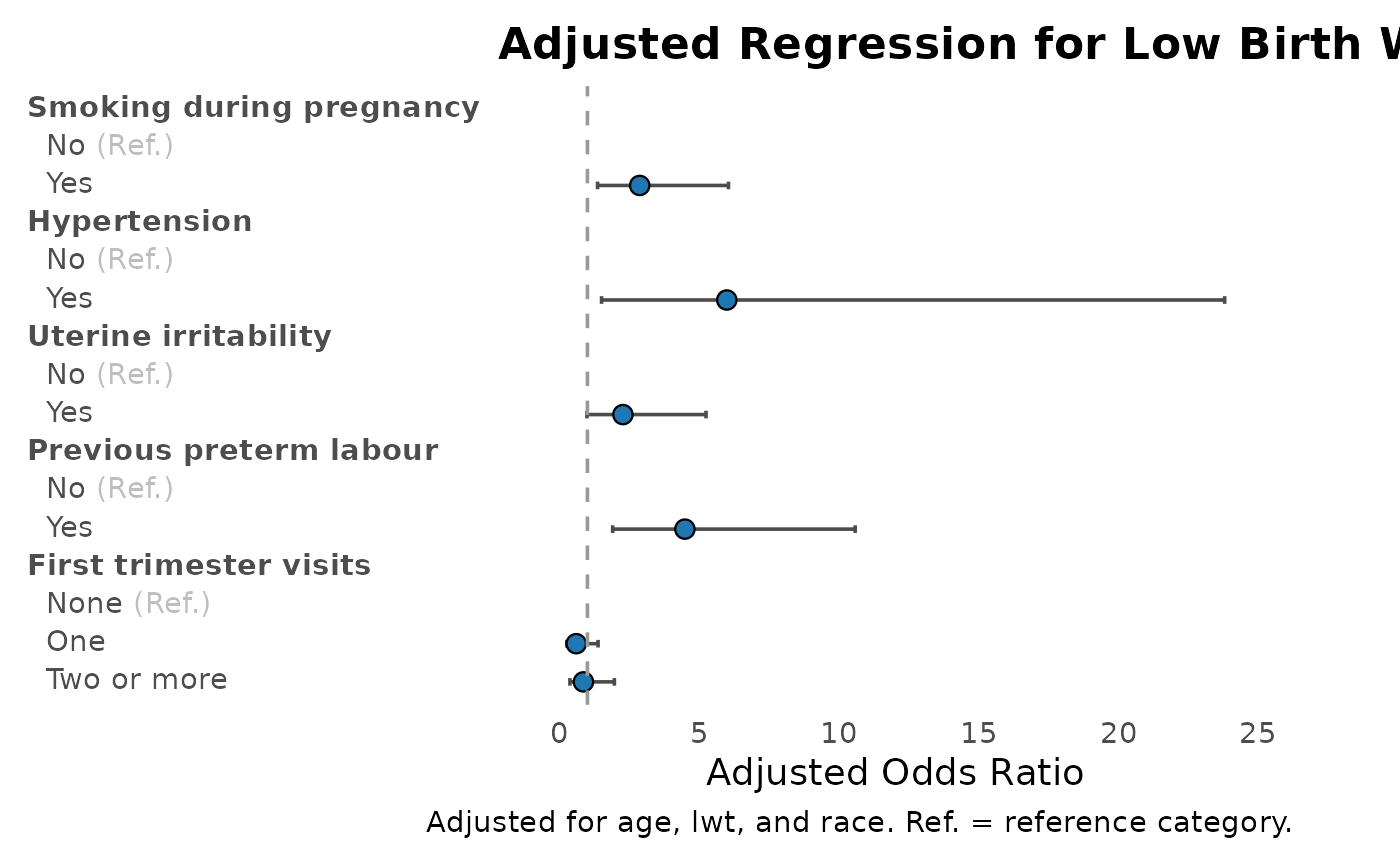
)
forest_reg(forest_df(birthwt_uni, birthwt_multi))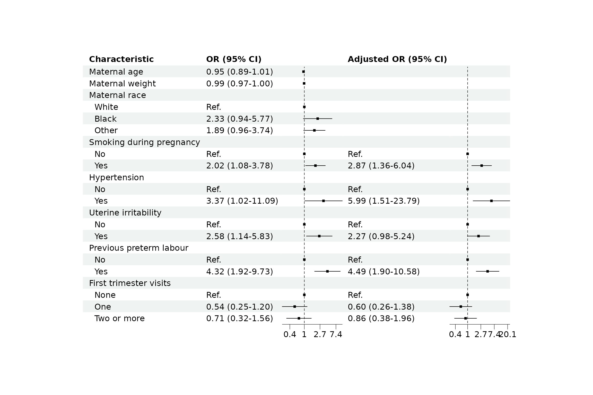
Merge and Polish
birthwt_final <- merge_tables(
  birthwt_summary,
  birthwt_uni,
  birthwt_multi,
  spanners = c("Clinical profile", "Crude OR", "Adjusted OR")
)

birthwt_final <- modify_table(
  birthwt_final,
  caption = "Clinical profile and regression estimates for low birth weight",
  caveat = "Adjusted estimates are adjusted for maternal age, maternal weight, and maternal race."
)

birthwt_final$table
Clinical profile |
Crude OR |
Adjusted OR |
||||||
|---|---|---|---|---|---|---|---|---|
Characteristic |
Normal BW |
Low BW |
Overall |
N |
OR (95% CI) |
p-value |
Adjusted OR (95% CI) |
p-value |
Maternal age |
23.0 (19.0-28.0) |
22.0 (19.5-25.0) |
23.0 (19.0-26.0) |
189 |
0.95 (0.89-1.01) |
0.105 |
||
Maternal weight |
123.5 (113.0-147.0) |
120.0 (104.0-130.0) |
121.0 (110.0-140.0) |
189 |
0.99 (0.97-1.00) |
0.023 |
||
Maternal race |
189 |
|||||||
White |
73 (56.2%) |
23 (39.0%) |
96 (50.8%) |
Ref. |
||||
Black |
15 (11.5%) |
11 (18.6%) |
26 (13.8%) |
2.33 (0.94-5.77) |
0.068 |
|||
Other |
42 (32.3%) |
25 (42.4%) |
67 (35.4%) |
1.89 (0.96-3.74) |
0.067 |
|||
Smoking during pregnancy |
189 |
|||||||
No |
86 (66.2%) |
29 (49.2%) |
115 (60.8%) |
Ref. |
Ref. |
|||
Yes |
44 (33.8%) |
30 (50.8%) |
74 (39.2%) |
2.02 (1.08-3.78) |
0.028 |
2.87 (1.36–6.04) |
0.006 |
|
Hypertension |
189 |
|||||||
No |
125 (96.2%) |
52 (88.1%) |
177 (93.7%) |
Ref. |
Ref. |
|||
Yes |
5 (3.8%) |
7 (11.9%) |
12 (6.3%) |
3.37 (1.02-11.09) |
0.046 |
5.99 (1.51–23.79) |
0.011 |
|
Uterine irritability |
189 |
|||||||
No |
116 (89.2%) |
45 (76.3%) |
161 (85.2%) |
Ref. |
Ref. |
|||
Yes |
14 (10.8%) |
14 (23.7%) |
28 (14.8%) |
2.58 (1.14-5.83) |
0.023 |
2.27 (0.98–5.24) |
0.055 |
|
Previous preterm labour |
189 |
|||||||
No |
118 (90.8%) |
41 (69.5%) |
159 (84.1%) |
Ref. |
Ref. |
|||
Yes |
12 (9.2%) |
18 (30.5%) |
30 (15.9%) |
4.32 (1.92-9.73) |
<0.001 |
4.49 (1.90–10.58) |
<0.001 |
|
First trimester visits |
189 |
|||||||
None |
64 (49.2%) |
36 (61.0%) |
100 (52.9%) |
Ref. |
Ref. |
|||
One |
36 (27.7%) |
11 (18.6%) |
47 (24.9%) |
0.54 (0.25-1.20) |
0.130 |
0.60 (0.26–1.38) |
0.230 |
|
Two or more |
30 (23.1%) |
12 (20.3%) |
42 (22.2%) |
0.71 (0.32-1.56) |
0.394 |
0.86 (0.38–1.96) |
0.717 |
|
Categorical variables shown as n (%); percentages are by column. | ||||||||
Continuous variables shown as Median (IQR). | ||||||||
Abbreviations: OR = Odds Ratio; CI = Confidence Interval. | ||||||||
Ref. = reference category. | ||||||||
Adjusted for Maternal age, Maternal weight, and Maternal race | ||||||||
N = 189 complete observations included in each adjusted model. | ||||||||
Adjusted estimates are adjusted for maternal age, maternal weight, and maternal race. | ||||||||
Save helpers return file paths and use tempdir() when no
directory is supplied, which keeps examples CRAN-safe.
save_table(birthwt_final, filename = "birthwt-table", format = html)
save_docx(tables = birthwt_final, filename = "birthwt-report")
Where To Go Next
- Descriptive Tables: build baseline tables users can read.
- Regression Tables: create crude and adjusted publication-ready outputs.
- Survival Analysis: Kaplan-Meier curves, survival summaries, Cox regression, parametric survival models, and survival predictions.
- Causal Mediation: estimate direct, indirect, total, and proportion mediated effects with clear causal caveats.
- Visualise Results: plot regression estimates and forest tables.
- Stratified Analysis: repeat models across subgroups.
- Diagnostics: check convergence, collinearity, and model selection.
- Confounding & Interaction: support interpretation and model decisions.
- Customize & Export: polish and save tables, plots, and reports.