Mediation analysis asks whether part of an exposure-outcome association may pass through an intermediate variable. In health research, that question is usually interesting only after the clinical story, temporal order, and likely confounding structure have already been considered.
gtregression provides a compact workflow for:
- fitting the mediator and outcome models;
- estimating total, direct, indirect, and proportion mediated effects;
- displaying a publication-style table;
- drawing a simple mediation path diagram.
The output is deliberately transparent. It is a model-based aid to interpretation, not proof of causality by itself.
Example Question
This article uses data_diabetes_mediation, a teaching
dataset based on a diabetes risk profile. The example question is:
Does plasma glucose explain part of the association between obesity and diabetes?
library(gtregression)
library(dplyr)

data("data_diabetes_mediation", package = "gtregression")

dissect(data_diabetes_mediation)Variable |
Type |
Missing (%) |
Unique |
Levels |
Compatibility |
Hint |
|---|---|---|---|---|---|---|
diabetes |
factor |
0% |
2 |
No, Yes |
compatible |
Factor variable can be used as categorical. |
obesity |
factor |
0% |
2 |
No, Yes |
compatible |
Factor variable can be used as categorical. |
glucose |
numeric |
0% |
90 |
- |
compatible |
Numeric variable can be used as continuous. |
bmi |
numeric |
0% |
200 |
- |
compatible |
Numeric variable can be used as continuous. |
age |
numeric |
0% |
49 |
- |
compatible |
Numeric variable can be used as continuous. |
blood_pressure |
numeric |
0% |
37 |
- |
compatible |
Numeric variable can be used as continuous. |
pregnancies |
numeric |
0% |
14 |
- |
compatible |
Numeric variable can be used as continuous. |
diabetes_pedigree |
numeric |
0% |
352 |
- |
compatible |
Numeric variable can be used as continuous. |
Screening aid only; review coding, missingness, sparse levels, and study context before modeling. | ||||||
Logistic Outcome
For a binary outcome, use outcome_approach = logit. The
effects are reported as predicted probability differences, which are
often easier to explain than odds ratios in a mediation table.
For final analyses, use a larger number of bootstrap simulations such
as sims = 500 or sims = 1000. The article uses
a smaller value to keep the example quick to run.
diabetes_med <- mediation_analysis(
  data = data_diabetes_mediation,
  exposure = obesity,
  mediator = glucose,
  outcome = diabetes,
  covariates = c(age, blood_pressure, pregnancies, diabetes_pedigree),
  outcome_approach = logit,
  sims = 100,
  seed = 123
)

diabetes_med
The returned object keeps the table body, fitted models, bootstrap draws, and exposure comparison values available for checking.
diabetes_med$table_body## effect Effect estimate conf.low conf.high
## total total Total effect 0.22624186 0.16258768 0.2907013
## direct direct Direct effect 0.17561583 0.11427535 0.2347698
## indirect indirect Indirect effect 0.05062603 0.01899140 0.0870712
## proportion proportion Proportion mediated 0.22376950 0.08741395 0.3821232
## p.value Interpretation
## total 0 Overall exposure-outcome association
## direct 0 Association not through the mediator
## indirect 0 Association through the mediator
## proportion 0 Share of total effect through the mediator
diabetes_med$values## $reference_value
## [1] "No"
##
## $exposure_value
## [1] "Yes"
diabetes_med$models$mediator##
## Call:
## stats::lm(formula = .mediation_formula(mediator, c(exposure,
## covariates)), data = df)
##
## Coefficients:
## (Intercept) obesityYes age blood_pressure
## 98.23467 6.66535 0.39847 0.06945
## pregnancies diabetes_pedigree
## 0.40874 5.56161
diabetes_med$models$outcome##
## Call: stats::glm(formula = f, family = stats::binomial(), data = df)
##
## Coefficients:
## (Intercept) obesityYes glucose age
## -6.848643 0.952467 0.034610 0.012419
## blood_pressure pregnancies diabetes_pedigree
## 0.003185 0.052420 0.590009
##
## Degrees of Freedom: 726 Total (i.e. Null); 720 Residual
## Null Deviance: 953.8
## Residual Deviance: 731.1 AIC: 745.1
head(diabetes_med$boot)## total direct indirect proportion
## 1 0.2299255 0.1705385 0.05938700 0.2582880
## 2 0.2550856 0.1917216 0.06336401 0.2484029
## 3 0.2126707 0.1747508 0.03791990 0.1783034
## 4 0.2907202 0.2280457 0.06267444 0.2155834
## 5 0.2906804 0.2387094 0.05197098 0.1787908
## 6 0.2486133 0.1939385 0.05467481 0.2199191Path Diagram
plot_mediation() draws the exposure, mediator, outcome,
and the direct and indirect paths.
plot_mediation(diabetes_med)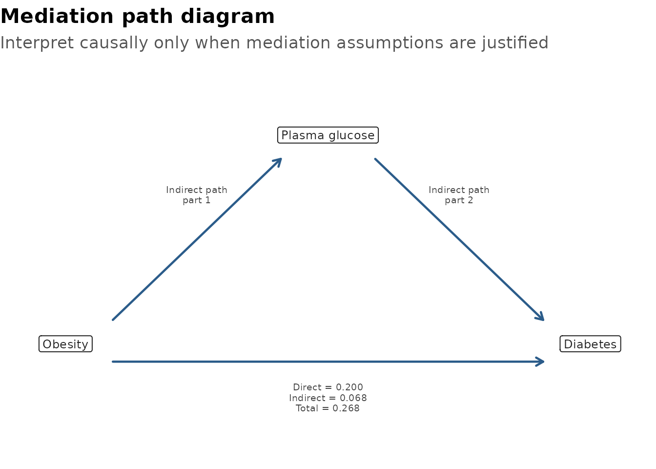
If the figure is being used only to explain the causal structure, hide the estimates.
plot_mediation(diabetes_med, show_estimates = FALSE)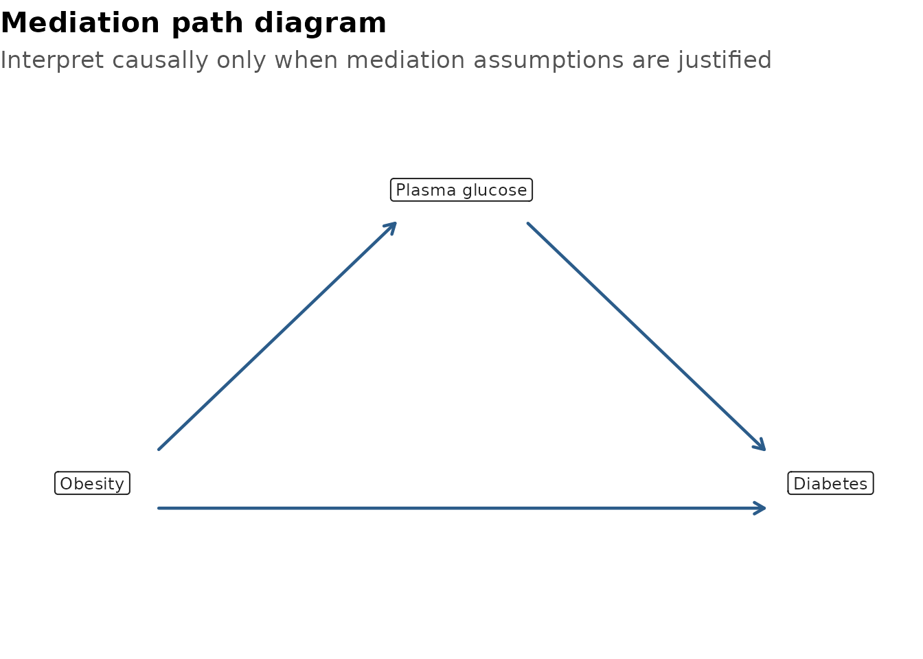
Quoted Names
Quoted column names and stored character vectors work too. This is useful inside scripts, functions, and Shiny-style workflows.
exposure_var <- "obesity"
mediator_var <- "glucose"
outcome_var <- "diabetes"
covariate_vars <- c(
  "age", "blood_pressure", "pregnancies", "diabetes_pedigree"
)

med_quoted <- mediation_analysis(
  data = data_diabetes_mediation,
  exposure = exposure_var,
  mediator = mediator_var,
  outcome = outcome_var,
  covariates = covariate_vars,
  outcome_approach = "logit",
  sims = 100,
  seed = 456
)

med_quoted
Linear Outcome
For a continuous outcome, use outcome_approach = linear.
In this example, the outcome is body mass index, so the effects are
reported as mean differences.
med_linear <- mediation_analysis(
  data = data_diabetes_mediation,
  exposure = obesity,
  mediator = glucose,
  outcome = bmi,
  covariates = c(age, blood_pressure, pregnancies, diabetes_pedigree),
  outcome_approach = linear,
  sims = 100,
  seed = 789
)

med_linear
plot_mediation(med_linear)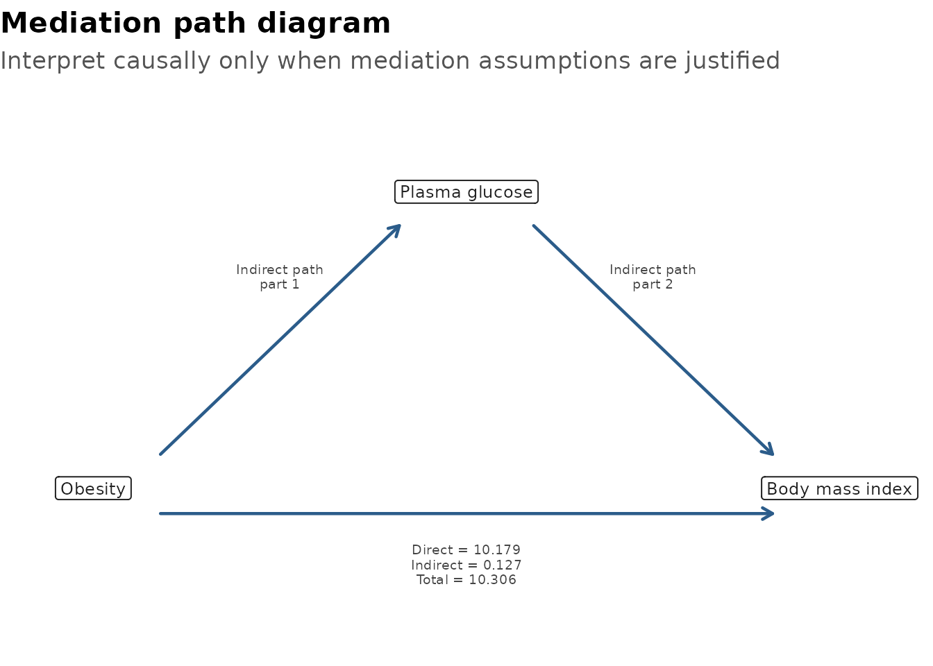
How To Report
A compact reporting sentence might look like this:
In this teaching analysis, plasma glucose explained part of the model-based obesity-diabetes association. Effects were estimated on the predicted probability difference scale using logistic outcome models and bootstrap confidence intervals.
The table footnote records the exposure comparison, mediator, outcome, bootstrap replicates, and adjustment variables so readers can see what was estimated.
What Not To Claim
Mediation estimates should not be treated as automatic causal proof. A cautious analysis should consider:
- whether the exposure clearly precedes the mediator;
- whether the mediator clearly precedes the outcome;
- whether exposure-mediator, mediator-outcome, and exposure-outcome confounding have been handled;
- whether post-exposure confounders are present;
- whether the model forms are plausible;
- whether a DAG or subject-matter argument supports the causal interpretation.
Use the table and plot to support interpretation after that thinking has been done.